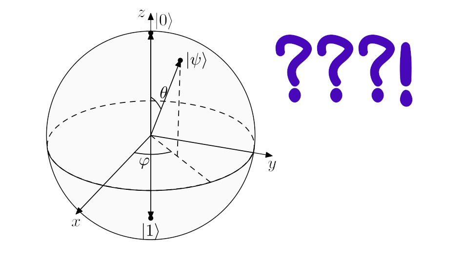
A bit is the smallest unit of information that there is. On or off. A 0 or a 1. Classical computers, like the kind you and I have, can be thought of as machines that manipulate lots of these bits in order to do useful stuff (or, at least stuff that you want it to do - you can be the judge of whether that’s useful or not).
But quantum computers? Well, they’re just cooler, right? I mean, look, it’s got quantum right there in the name. Even their bits are cool. Because quantum bits- wait, no… ~qubits~ (yeah, that sounds cool) can even be 0s and 1s at the same time!…I mean, kinda. Sorta. How?
When it comes to quantum computers, there’s a lot of popular science that doesn’t go much beyond this. And, if you do go looking for something more substantial, there’s a decent amount of higher-level, computer science stuff about quantum algorithms, but very little in the quite frankly massive gulf between these two options. So I thought I’d write about the qubit. Just the qubit. What it is and how it works.
I’ll also talk about the Bloch sphere, a way of representing qubit states that gets thrown at you very often very early with no explanation as to why it’s used or why it looks like that. Again, it is difficult to find explanations between the extremes of ‘substitute these trig identities and carry on’ and ‘hope you know your 4D topology’, so I’ve tried to find a kind of “middle-ground” explanation to bridge the gap.
You don’t need an extensive maths background to read this, and you don’t need to know any quantum mechanics as I’ll introduce it here. You should be comfortable manipulating simple algebraic expressions and know some basic trigonometry, and ideally you’re comfortable with using radians to measure angles and know some simple vector operations. I’m in the UK, so I’ll say that if you have a strong maths GCSE you’ll probably be fine, and if you have a maths A-level you’ll definitely be fine. Let’s go!
Bits
Classical bits are simple. A bit can exist in one of two states: we often call these the 0 state, and the 1 state, though really we could call them anything. 0 and 1 might represent low voltage and high voltage in a circuit, an uncharged and charged capacitor, or any other system with two states. The use of 0 and 1 is just an abstraction of these physical objects.
Qubits can be measured as being in one of two eigenstates: we often call these the \(\ket{0}\) state, and the \(\ket{1}\) state, though really we could call them anything. \(\ket{0}\) and \(\ket{1}\) might represent the spin-up and spin-down state of an electron, the ground state and first excited state of a particle, or any other quantum system with two eigenstates. The use of \(\ket{0}\) and \(\ket{1}\) is just an abstraction of these physical systems.
You might be wondering why \(\ket{0}\) and \(\ket{1}\) are in those funny angle brackets. These are used to denote that \(\ket{0}\) and \(\ket{1}\) are vectors. Representing eigenstates as vectors is useful for a few reasons, one of which is because of a property of quantum systems known as superposition.
We always measure a quantum system as being in just one eigenstate, though, up until we measure it, it may exist in a superposition of eigenstates. A superposition is a kind of combination of states. In fact, it’s really just the physics word for a linear combination. If you don’t know what a linear combination is, then it’s just a way of adding vectors together. For example, we could create a new vector, let’s call it \(\ket{\psi}\), like this:
\[\ket{\psi} = a\ket{0} + b\ket{1}\]and we would say that \(\ket{\psi}\) is in a superposition of \(\ket{0}\) and \(\ket{1}\). \(a\) and \(b\) here represent the amount of \(\ket{0}\) and \(\ket{1}\) that \(\ket{\psi}\) is made up of. For example, a large value for \(a\) and a small value for \(b\) would produce a vector that points mostly in the same direction as \(\ket{0}\).
\(\ket{\psi}\) is the symbol we normally give to the current state of a quantum system, so the equation above is how we represent our qubit being in a superposition of eigenstates. In the interaction below, you can see how the values of \(a\) and \(b\) change as we change the vector \(\ket{\psi}\).
From this interaction, we can see that we can think about \(a\) and \(b\) as the ‘projection’ of \(\ket{\psi}\) onto \(\ket{0}\) and \(\ket{1}\). If you know some trigonometry, you’ll notice that this means we can get the values of \(a\) and \(b\) by taking the cosine of the angle between \(\ket{\psi}\) and \(\ket{0}\) and \(\ket{1}\) respectively. If you know some vector maths, you’ll notice that this means we can also get these values by performing the dot product of \(\ket{\psi}\) with these vectors.
Something you’ll notice is that when \(\ket{\psi}\) is in an eigenstate (that is, when it lies entirely in either the \(\ket{0}\) or \(\ket{1}\) direction), its projection onto that state becomes 1, and its projection onto the other state becomes 0. Earlier, we said that a quantum system can only ever be measured as being in a single eigenstate, not a superposition, so this makes sense! If this weren’t the case, then when \(\ket{\psi}\) is in an eigenstate, its projection onto the other state would be non-zero, meaning it would still be in a superposition! A property of quantum eigenstates is that they are always orthogonal, which is what prevents this from happening. We say states are orthogonal when they have 0 projection onto each other, which is why \(\ket{0}\) and \(\ket{1}\) are drawn at right-angles to each other above.
Finally, you probably noticed that the values of \(a\) and \(b\) are never greater than 1. This is due to what \(a\) and \(b\) represent physically. We know that \(\ket{\psi}\) must always collapse into an eigenstate upon measurement - \(a\) and \(b\) actually tell us the probability of \(\ket{\psi}\) collapsing into either \(\ket{0}\) or \(\ket{1}\). This means that the ‘closer’ \(\ket{\psi}\) is to \(\ket{0}\) or \(\ket{1}\), the higher the probability of measuring it in that state. The Born rule is a postulate of quantum mechanics that says that, specifically, the probability is given by the size of these values squared:
Probability of measuring \(\ket{0} = \lvert a \rvert^{2}\)
Probability of measuring \(\ket{1} = \lvert b \rvert^{2}\)
As total probabilities must always add up to 1, this means we have the following constraint on our system:
\[\lvert a \rvert^{2} + \lvert b \rvert^{2} = 1\]This is why the state vector \(\ket{\psi}\) always has a length of 1!
Because of their relation to probability, we call \(a\) and \(b\) probability amplitudes.
The wavefunction
…But why amplitudes? I guess we can’t just call them probabilities, because we have to do something to them first to get the probability out, but amplitudes?
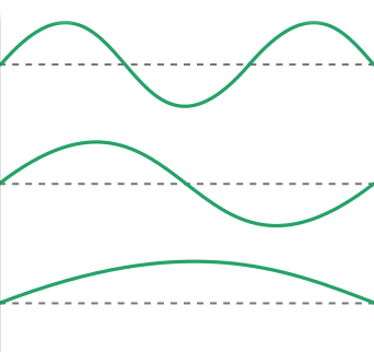
If you’ve ever studied some quantum mechanics, you’ve probably met \(\psi\) before, but you may not have met it as the vector \(\ket{\psi}\). In fact, most people are introduced to \(\psi\) as the wavefunction, \(\psi(x)\). As it’s a function, we can plot it. You might have seen it look something like one of these:
Or maybe something a little more realistic, with more dimensions, like this:
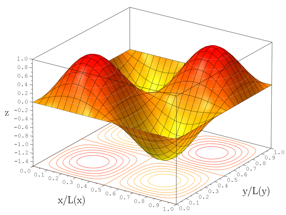
Of course, exactly what the plot \(\psi(x)\) looks like will be different depending on which physical system our qubit is constructed from, but it will always be made up of a linear combination (a superposition) of eigenfunctions.
Hmm, this sounds familiar. Could it be that \(\psi(x)\) is a superposition of eigenfunctions in the same way that \(\ket{\psi}\) is a superposition of eigenvectors?
Yes! In fact, the function \(\psi(x)\) is the vector \(\ket{\psi}\). I’ll say it again: \(\psi(x)\) and \(\ket{\psi}\) are the same object. This can be true because all functions are vectors. This is not intuitive, but it is an important point. If you’d like to know more about how functions are vectors, then this entry from a previous SoME is excellent.
Naturally then, it follows that the eigenstates \(\ket{0}\) and \(\ket{1}\) can also be drawn as functions. Here is an example of two possible energy eigenstates - a ground state, and an excited state:
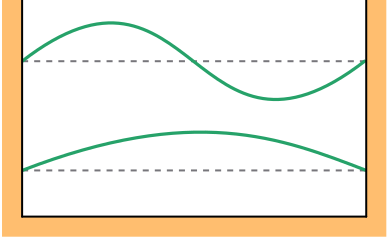
You’ll notice that these functions are waves. With amplitudes! In fact, when we combine \(\ket{0}\) and \(\ket{1}\) to create \(\ket{\psi}\), \(a\) and \(b\) in this equation:
\[\ket{\psi} = a\ket{0} + b\ket{1}\]are the amplitudes of these waves! This is the reason why \(a\) and \(b\) are called probability amplitudes - they are the literal amplitudes of these eigenstates! In the interaction below, you can change the values of \(a\) and \(b\) to see how this changes the shape of the wavefunction \(\ket{\psi}\).
Adding Complexity
I must now confess that I have told you a lie. Or, well, more that I have omitted a truth. The functions above aren’t actually static, like I’ve shown them - they evolve over time. Specifically, they rotate, like this:
This of course means that \(a\) and \(b\), their amplitudes, must rotate. But how do we keep track of this rotation? A single number surely won’t do it!
Well, perhaps a single real number won’t do it. The real numbers are the ones that lay on the number line, like this:

Using the real numbers, there is one specific kind of rotation we can do - a rotation of 180°. We do this by flipping the sign, which is what happens when we multiply by -1.
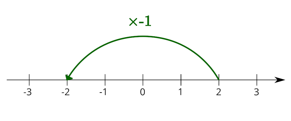
But, in order to see a rotation by any other angle, we need at least 2 dimensions - more than just the single dimension that the real number line gives us. The special number \(i\) is a number that rotates by 90° when we multiply by it. Because two 90° rotations make a 180° rotation, we know that multiplying by \(i\) twice is the same as multiplying by -1, so therefore \(i^2 = -1\), or \(i = \sqrt{-1}\).
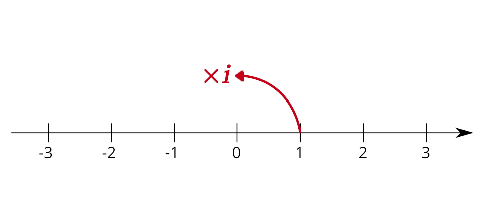
\(i\) is what we call an imaginary number. Because multiplying by imaginary numbers rotates by 90°, we can visualise them as laying on an ‘imaginary’ number line perpendicular to the real number line. We can now use these two number lines to describe a set of 2-dimensional numbers which we can use for our rotations - we call these the complex numbers.
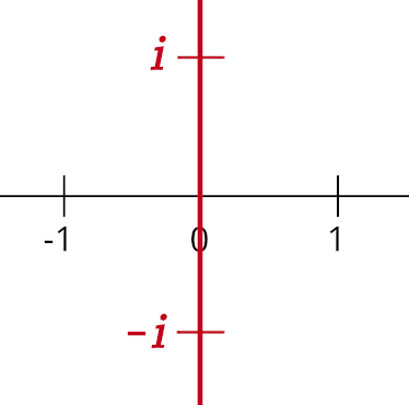
Complex numbers are numbers that have a real component and an imaginary component. We could write some complex number \(z\) like this:
\[z = \alpha + \beta i\]where \(\alpha\) is the real part and \(\beta\) is the imaginary part. We can visualise them as laying on a plane:
However, as we’re interested in rotations, there’s also a different way we can write them that will be more useful to us. Instead of writing out their real and imaginary parts explicitly, we could instead write them using their magnitude (their distance from 0), and the angle they make with the real axis. Click the button on the interaction above to see how \(z\) looks when written in this form.
…Okay, but why is that \(e\) there?! Great question! \(e\) is actually shorthand for a function named \(\exp()\), called the exponential function, and its exponent is the value we input into that function, so \(e^{i \theta} = \exp(i \theta)\). The form of the \(\exp()\) function means that, when we input a number multiplied by \(i\), it acts as a combination of the sine and cosine functions, which is what causes the rotation.
Because it only controls rotation, and not magnitude, we call \(\exp(i \theta)\) the phase of the state.
Interference
Okay, so let’s recap: \(\ket{\psi}\) is a quantum state made up of a superposition of two eigenstates \(\ket{0}\) and \(\ket{1}\). \(a\) and \(b\) are the amplitudes of the functions \(\ket{0}\) and \(\ket{1}\) - these amplitudes rotate over time, so \(a\) and \(b\) are complex numbers in order to describe this rotation. \(a\) and \(b\) also give us the probability of measuring \(\ket{\psi}\) as being in either the \(\ket{0}\) or \(\ket{1}\) state.
…Wait, hang on. \(a\) and \(b\) rotate and are complex but are also probabilities?! How does that even work? What does it mean for probabilities to rotate?!
Well, remember that \(a\) and \(b\) aren’t probabilities by themselves - they’re actually just probability amplitudes. We can’t measure probability amplitudes, just probabilities, which are given by \(\lvert a \rvert^{2}\) and \(\lvert b \rvert^{2}\). The notation \(\lvert a \rvert\) and \(\lvert b \rvert\) means that we only care about the magnitude of \(a\) and \(b\), meaning that, when we measure this probability, we lose the phase information anyway.
What?! So why does it matter, then? Was all that work for nothing?! How do we even know \(a\) and \(b\) rotate if we can’t measure the rotation?!
It’s true that we actually don’t know the rotation of a particular state, what we call the global phase, but that doesn’t mean it doesn’t matter. Something that we can measure is the difference in rotation between two states. We call this the relative phase, and we can detect it because it changes how the \(\ket{0}\) and \(\ket{1}\) states add together, or interfere with each other, which changes the shape of the resulting wavefunction.
Even though we can’t detect the wavefunction directly, its shape matters because it determines how the qubit will behave when we perform operations on it, like applying quantum logic gates. You may have been wondering how we ever get any information out of a quantum computer if every measurement is probabilistic. This interference of states is how. Programming a quantum computer involves applying quantum logic gates in such a way that all the outcomes you don’t want to see to destructively interfere with each other, or cancel out, so that you have the highest probability of measuring the correct answer.
The Bloch Sphere
At the beginning of this article, I showed you how we could think of \(\ket{\psi}\) as being projections onto \(\ket{0}\) and \(\ket{1}\), with \(a\) and \(b\) being the size of these projections:
But, now we know that this is a bit of a simplification. \(a\) and \(b\) can’t be represented as one-dimensional numbers like this; they’re complex, meaning we need two dimensions to represent each of them. This means that we need a total of four dimensions in order to represent both.
…Hmm, this is a problem. Unfortunately, we only live in three dimensions, so we can’t visualise four dimensions very well at all (well, I suppose there’s a chance you can, but I certainly can’t). So how are we meant to have a good way of representing all of our qubit states??
The answer is something called the Bloch sphere, which I will show to you now:
You may notice it has some familiar elements. We still have our state vector \(\ket{\psi}\), for example. And \(\ket{0}\) and \(\ket{1}\) are still there, albeit in a rather… strange position.
But mostly it looks quite different. There are more dimensions, which we expected (though how are we getting away with only 3?), and, oh yeah, what’s that sphere doing there???
First, let’s look at the dimensionality. We know \(a\) and \(b\) are complex numbers, so let’s write them out in their complex exponential form, as a magnitude and a phase:
\[a = r_a e^{i\phi_a}\] \[b = r_b e^{i\phi_b}\]which makes \(\ket{\psi}\) equal to:
\[\ket{\psi} = r_a e^{i\phi_a} \ket{0} + r_b e^{i\phi_b} \ket{1}\]Here, we can see that we have four different things to keep track of: \(r_a, \phi_a, r_b, \phi_b\). This is why we need four dimensions. If we want to reduce the number of dimensions we need, we somehow need to track fewer things. But how?
In the last section, we spoke about the difference between global phase, which we can’t measure, and relative phase, which we can. As global phase has no physical significance, any time it shows up, we can ignore it.
What does that mean for us? It means that we don’t actually care about the individual phases of \(a\) and \(b\), \(e^{i\phi_a}\) and \(e^{i\phi_b}\), we only care about their phase difference, \(e^{i(\phi_b - \phi_a)}\). This lets us reduce the number of variables from four down to just three: \(r_a\), \(r_b\), and \((\phi_a - \phi_b)\) which, for simplicity, I’ll now write simply as \(\phi\). Mathematically, what we’re doing is factoring out \(e^{i\phi_a}\). As it multiplies the entire expression, this is the global phase, which we can ignore.
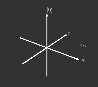
\[\ket{\psi} = e^{i\phi_a}(r_a \ket{0} + r_b e^{i(\phi_b - \phi_a)} \ket{1})\] \[\ket{\psi} = r_a \ket{0} + r_b e^{i\phi} \ket{1}\]This gets us down to just 3 dimensions. We can have the z-axis representing the real coefficient of \(\ket{0}\), \(r_a\), and the x-y plane representing the complex coefficient of \(\ket{1}\), \(r_b e^{i\phi}\):
The… Sphere?
Great! But, where does the sphere come into it? It is the Bloch sphere after all. Well, remember from earlier that \(\ket{\psi}\) must always have a magnitude of 1, due to the fact that the probabilities \(\lvert a \rvert^{2}\) and \(\lvert b \rvert^{2}\) must always add up to 1. This means that it’s confined to the set of points located at a distance of exactly 1 from the origin - in three dimensions, this is a sphere!
So, there we have it. The Bloch sphere:
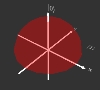
Hang on, that can’t be right. That’s only half a sphere! What’s going on?
Well, remember when we factored out the phase \(e^{i\phi_a}\) we left behind just the magnitude of the original \(\ket{0}\) coefficient: \(r_a\). Magnitudes are always positive, meaning we don’t use the negative half of the z-axis.
So, why is it the Bloch sphere, then? Why not just name it the Bloch hemisphere and call it a day?
The problem is, it actually is, topologically, a sphere! How? Let’s take a look at a qubit that lays entirely in the \(\ket{0}\) state:
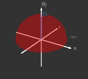
It points straight up, right? This means that the state \(\ket{\psi} = \ket{0}\) only has a single representation on the Bloch sphere, no matter what the value of \(\phi\) is. This is how it should be, as when a qubit lays entirely in an eigenstate there is no relative phase, as the other component goes to 0.
Now look at a qubit that lays entirely in the \(\ket{1}\) state:
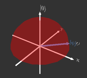
It should be the same as in the \(\ket{0}\) state, independent of \(\phi\), but in this pseudo-Bloch hemisphere it isn’t. Instead, we have this entire circle of states all representing the same physical state, \(\ket{\psi} = \ket{1}\). This whole circle should be collapsed to a single point, as it all represents a single state.
So how do we get our sphere? First, as we’re working with a sphere,let’s alter our equation for \(\ket{\psi}\) slightly to use spherical coordinates. This involves rewriting \(r_a\) and \(r_b\) in terms of the angle that \(\ket{\psi}\) makes with the z axis, which we’ll call \(\gamma\):
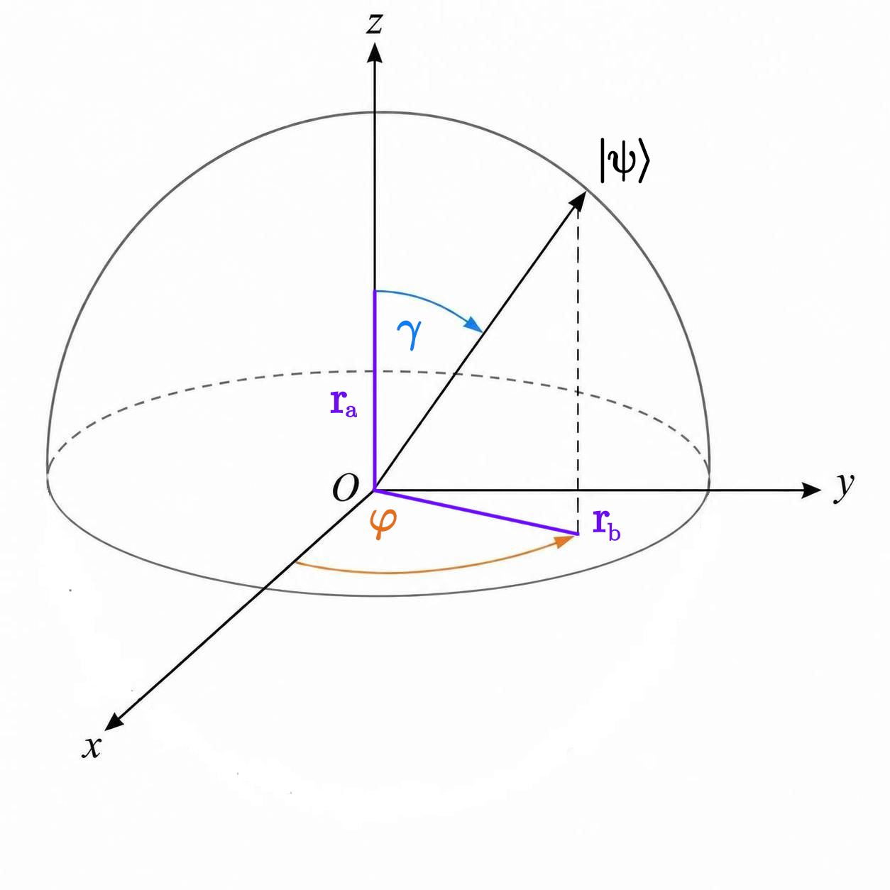
This means we can write \(\ket{\psi}\) as:
\[\ket{\psi} = \cos\gamma\ket{0} + e^{i\phi}\sin\gamma \ket{1}\]Because we’re just rewriting what we already had, the angle \(\gamma\) will only take us 90°, forming the hemisphere. However, we can do something sneaky, and define another angle, let’s call it \(\theta\), which is always double whatever \(\gamma\) is: \(\theta = 2\gamma\).
This way, when \(\gamma\) gets to 90°, \(\theta\) reaches all the way to 180, forming a sphere. This also means that the entire \(\ket{1}\) plane collapses to a single point opposite that of \(\ket{0}\) on the z-axis, exactly like we wanted!:
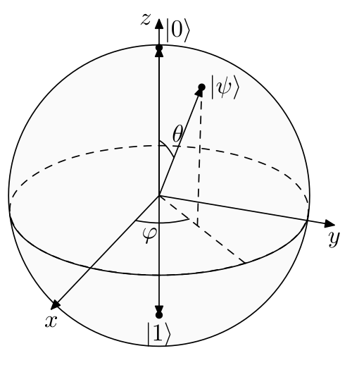
We just need to be careful to divide by 2 again when writing out \(\ket{\psi}\):
\[\ket{\psi} = \cos\frac{\theta}{2}\ket{0} + e^{i\phi}\sin\frac{\theta}{2} \ket{1}\]